![]()
Personalizing drug doses
in the cloud using R
Gergely Daróczi
Co-founder, CTO
Rx Studio Inc.
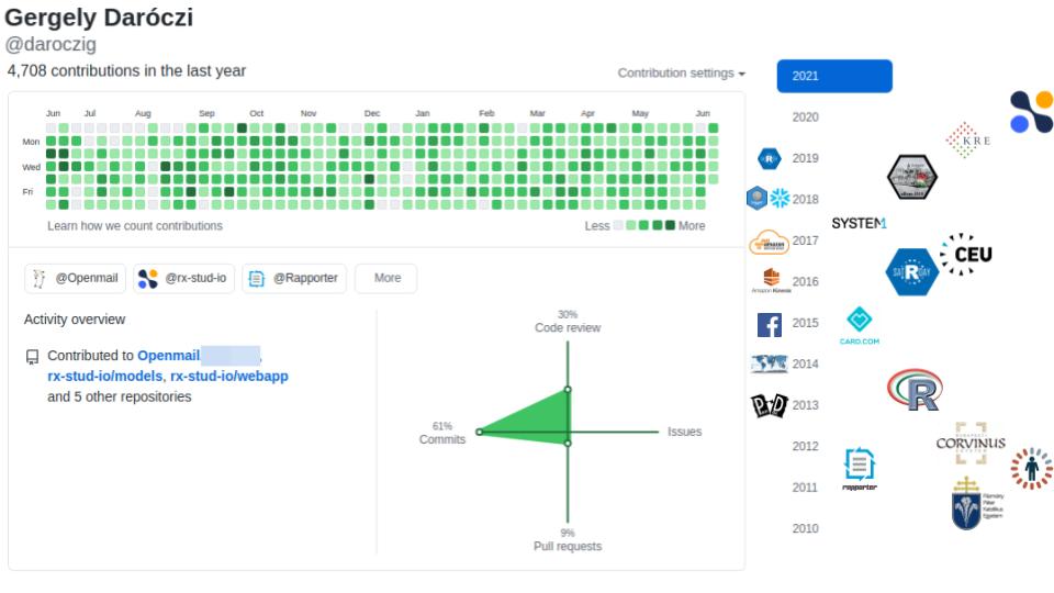
$ whoami

$ whoami
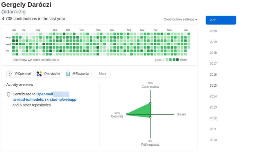
$ whoami

$ whoami

$ whoami

$ whoami
$ pwd

$ lsb_release

$ lsb_release

Source:
When
my co-worker wants to simplify code
that took two days to
understand
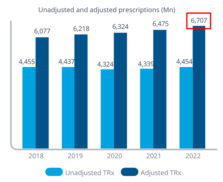
> Sys.getenv(country = ‘USA’)

Source: The Use of Medicines in the U.S. 2023 (IQVIA)
> Sys.getenv(country = ‘USA’)
> Sys.getenv(country = ‘USA’)
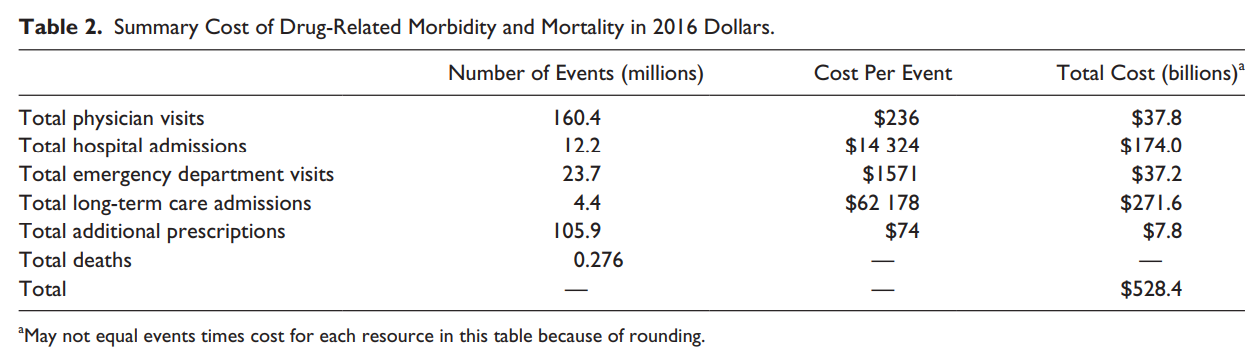
The estimated annual cost of prescription drug–related morbidity and mortality resulting from nonoptimized medication therapy was $528.4 billion in 2016 US dollars. Watanabe et al, 2018 (doi.org/10.1177/10600280187651)
> Sys.getenv(country = ‘USA’)
If medications were prescribed, monitored and taken properly,
we wouldn’t face this cost, and patients would be healthier. Watanabe et al, 2018 (doi.org/10.1177/10600280187651)
> ??properly

> demo(‘rx.studio’)

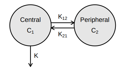
> vignette(topic = ‘PK/PD models’)
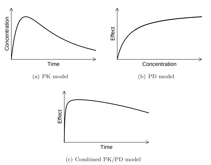
> vignette(topic = ‘PK/PD models’)

Source: Mortensen et al (2008): Introduction to PK/PD modelling.
> vignette(topic = ‘PK/PD models’)
Source: Mortensen et al (2008): Introduction to PK/PD modelling.
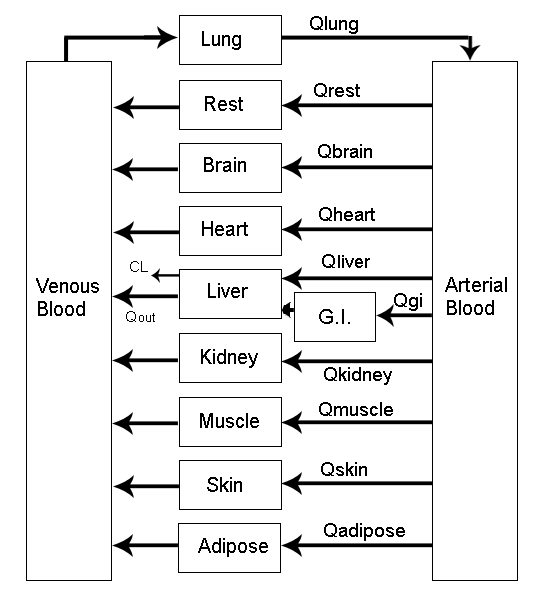
> vignette(topic = ‘PK/PD models’)
Source: Mortensen et al (2008): Introduction to PK/PD modelling.
> vignette(topic = ‘PK/PD models’)
Source: Mortensen et al (2008): Introduction to PK/PD modelling.
> vignette(topic = ‘PK/PD models’)

Source: Spherical cow
> vignette(topic = ‘PK/PD models’)
> vignette(topic = ‘PK/PD models’)
\[C=\frac{A}{V}\]
- \(C\) drug concentration
- \(A\) drug amount
- \(V\) volume of distribution
Example: 500 mg Panadol (\(Vd = 0.9L/kg\)) administered for a 70 kg patient
\[C=\frac{500mg}{70kg * 0.9L/kg}=\frac{500mg}{63L}=7.9 mg/L\]
> vignette(topic = ‘PK/PD models’)
> vignette(topic = ‘PK/PD models’)
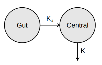
\[C_{oral}(t)=\frac{A_{oral}(t)}{V}=\frac{K_aFA_0}{V(K_a-K)}(exp(-K \cdot t) - exp(-K_a \cdot t))\]
- \(C\) drug concentration
- \(A\) drug amount
- \(V\) volume of distribution
- \(K_a\) absorption constant
- \(K\) elimination rate
- \(F\) bioavailability
> vignette(topic = ‘PK/PD models’)
![]()
\[C_{oral}(t)=\frac{A_{oral}(t)}{V}=\frac{K_aFA_0}{V(K_a-K)}(exp(-K \cdot t) - exp(-K_a \cdot t))\]
#' Concentration at a time computed using a one-compartment model (oral dose)
#' @param t time (hours)
#' @param dose dose amount (mg)
#' @param v volume of distribution (l)
#' @param k elimination rate constant (h^-1)
#' @param ka absorption rate constant (h^-1)
#' @param f bioavailability
#' @return numeric
#' @export
ct <- function(t, dose, v, k, ka, f) {
    (ka * f * dose) / (v * (ka - k)) * (exp(-k * t) - exp(-ka * t))
}
> example(topic = ‘paracetamol’)

Source: Rawlins et al. (1977): Paracetamol (simplified)
> example(topic = ‘paracetamol’)

Source: Rawlins et al. (1977): Paracetamol (simplified)
> example(topic = ‘paracetamol’)
library(data.table); library(ggplot2)
conc <- data.table(h = seq(0, 24, by = 0.1))
conc[, c := ctp(h, 1000)]
ggplot(conc, aes(h, c)) + geom_line()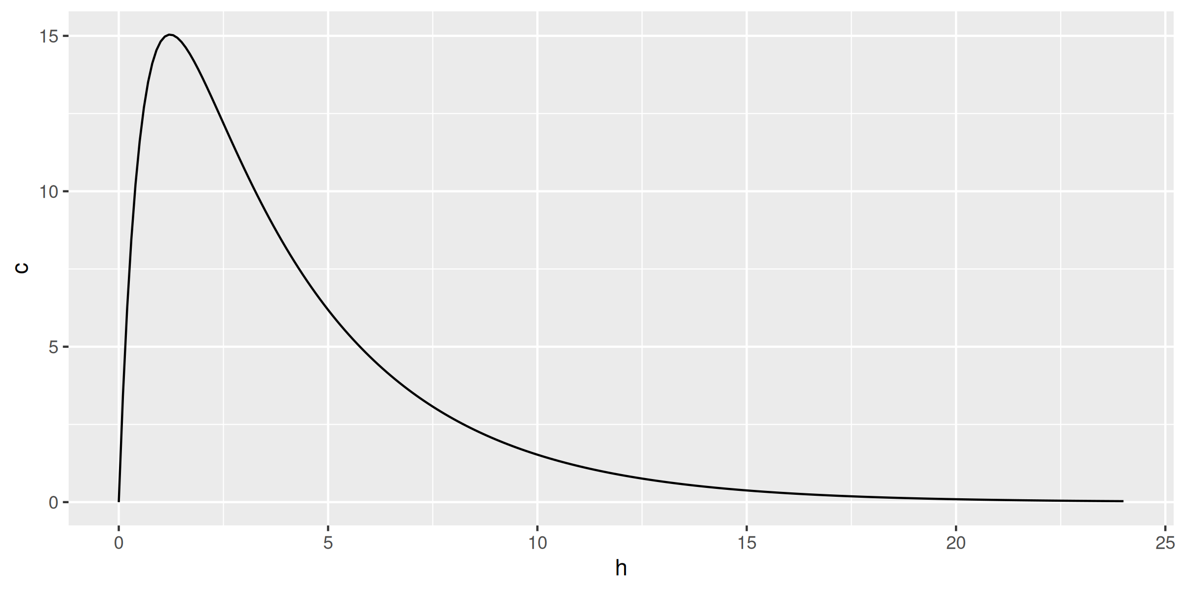
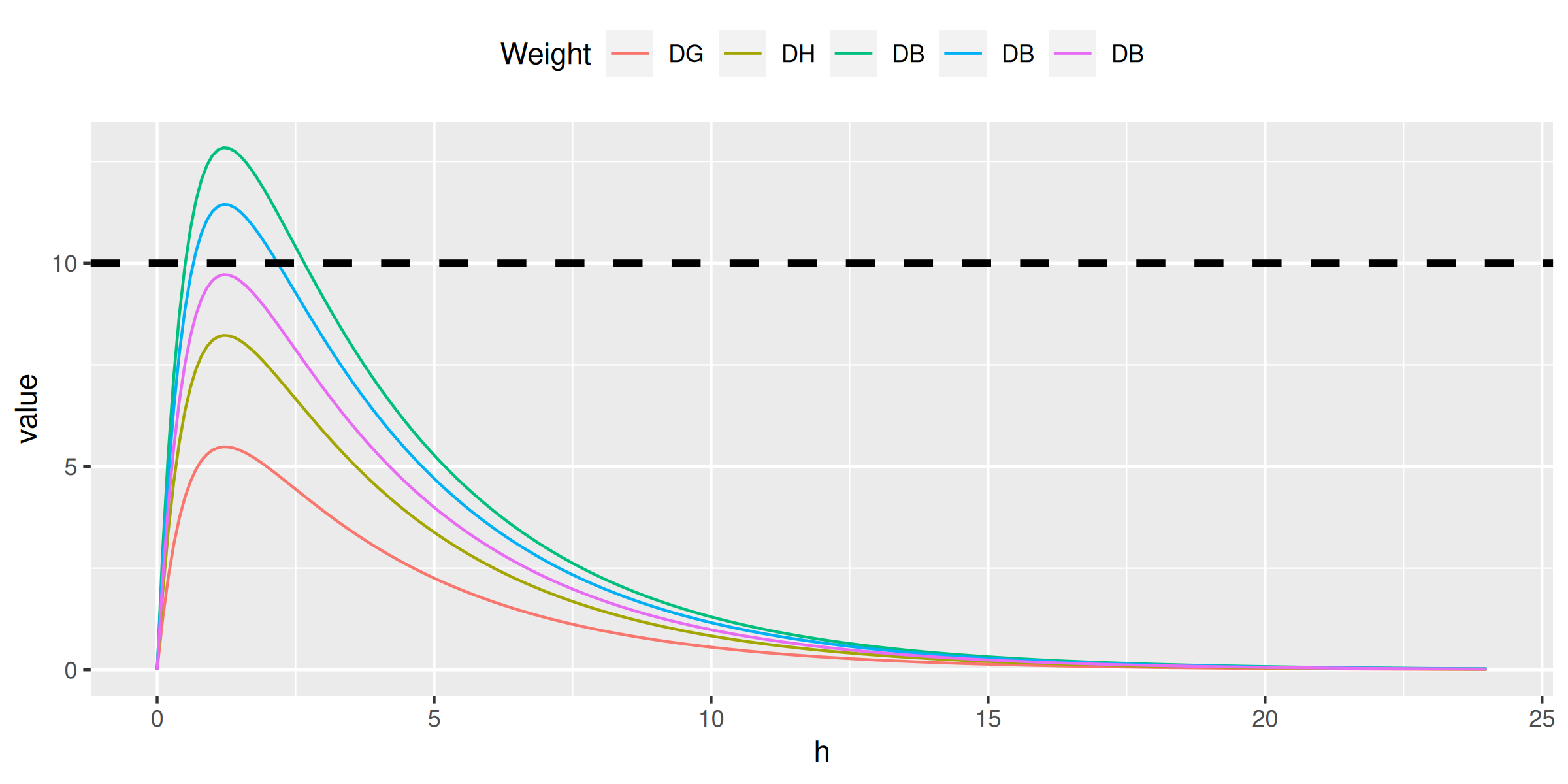
> do.call(ctp, weights)

> do.call(ctp, family)
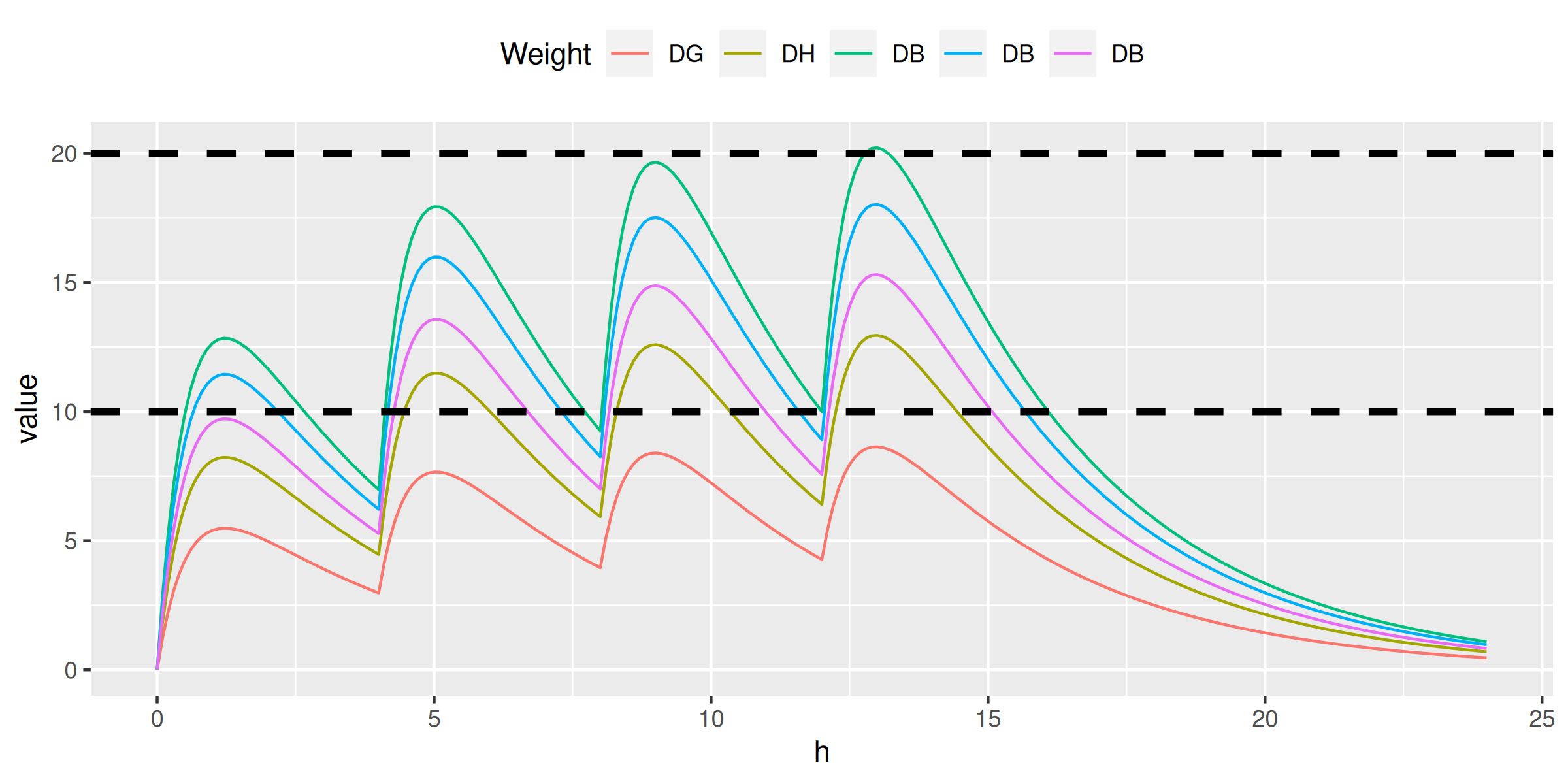
> do.call(ctp, family, ndoses = 4)
> sd(do.call(ctp, rlnorm(2000)))
Source: Rawlins et al. (1977): Paracetamol (simplified)
> sd(do.call(ctp, rlnorm(2000)))
weight <- 70
meanlog <- log((weight * 0.6)^2 / sqrt(0.07^2 + (weight * 0.6)^2))
sdlog <- sqrt(log(1 + (0.07^2 / (weight * 0.6)^2)))
ggplot(data.frame(x = rlnorm(n = 2000L, meanlog, sdlog))) +
    geom_histogram(aes(x)) +
    ggtitle('Volume of distribution for 70 kg') + xlab('')
> sd(do.call(ctp, rlnorm(2000)))
for (i in 1:250) {
   meanlog <- log((weight * 0.6)^2 / sqrt(0.07^2 + (weight * 0.6)^2))
   sdlog <- sqrt(log(1 + (0.07^2 / (weight * 0.6)^2)))
   conc <- copy(conc)[, c := ct(h, 1000, v = rlnorm(n = 1L, meanlog, sdlog),
                                k = 0.28, ka = 1.8, f = 0.89)]
   (G <- G + geom_line(data = conc, color = 'gray', alpha = 0.1))
}
G + geom_line(color = 'black') + ggtitle('250 simulations')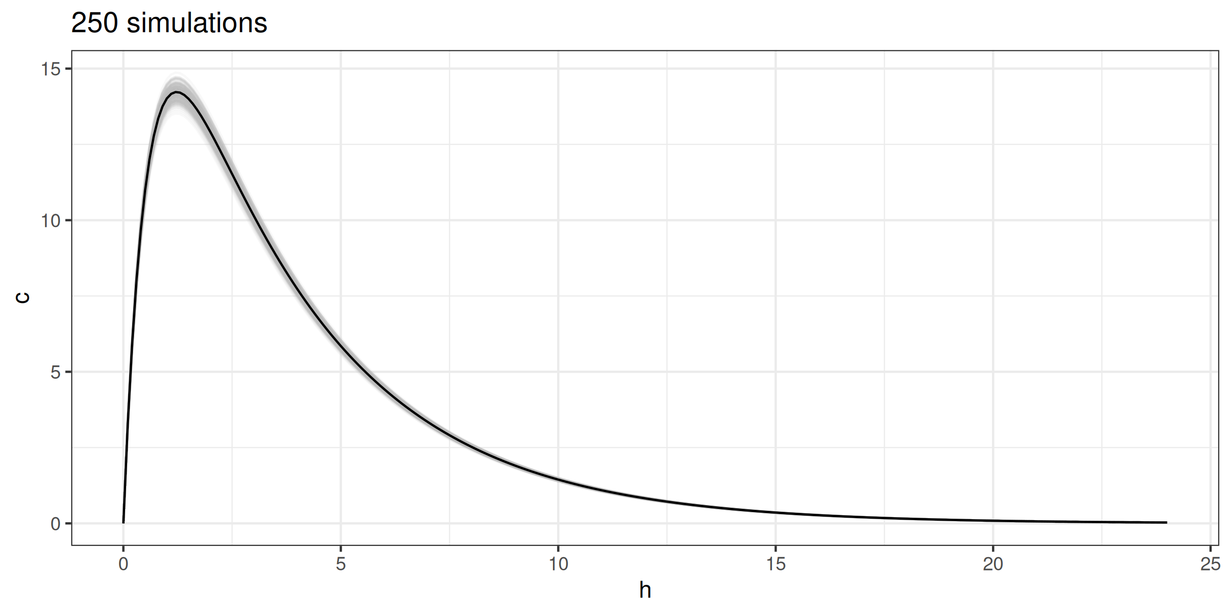
> sd(do.call(ctp, rlnorm(2000)))

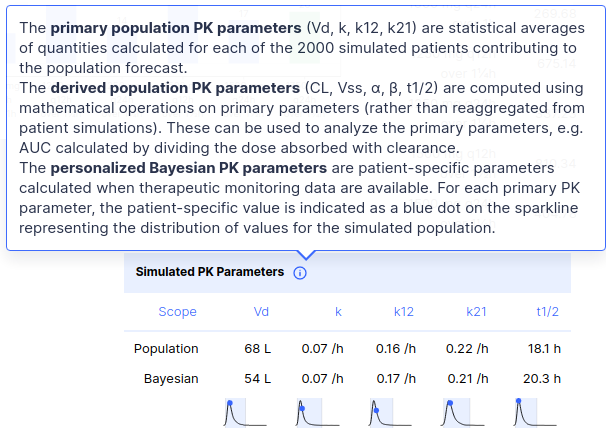
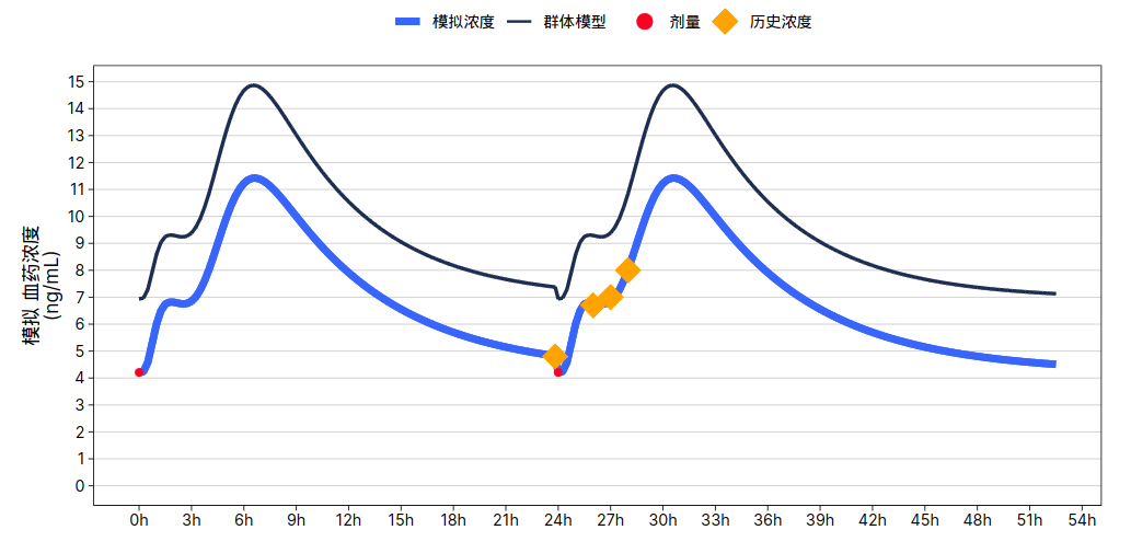
> fit(ctp, data.frame(conc = 5))
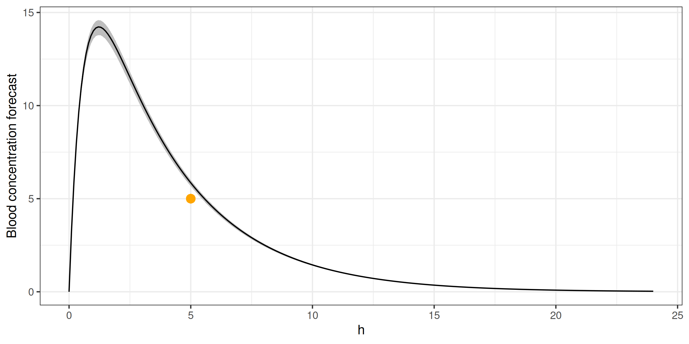
> fit(ctp, data.frame(conc = 5))
> 0.60 * 70
[1] 42
> bay$par[['v']]
[1] 51.954
> fit(ctp, data.frame(conc = 5))
> fit(ctp, data.frame(conc = 5))
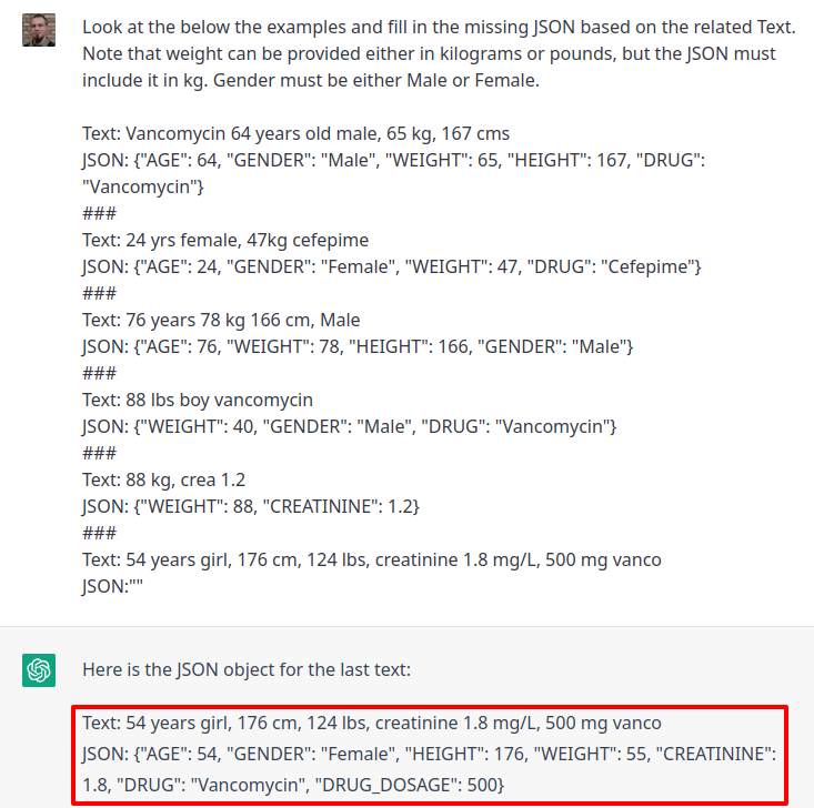
> library(chatgpt)
![]()
> library(chatgpt)
![]()
> library(chatgpt)
![]()
> library(chatgpt)

> library(chatgpt)

> library(chatgpt)
placeholder as cannot finish with an image