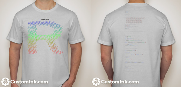
Pull requests for user2014/t-shirt:

#1 by jimhester: original idea

#2 by @daroczig: using pixmap to create ASCII art

#3 by @bryanhanson: Bayes Icon

#4 by @fhoces: CLT with R

#5 by @MarkTPatterson: EBImage package

#6 by @calycolor: wordcloud

#8 by @woobe: RShapeTarget package

#9 by @hanel: ggplot2

#10 by @royfrancis

#11 by @notesofdabbler

#1 by @jimhester

recycled lengths rather than repeated calls to rep
formatted lens specification by row
use strsplit of character string rather than explicit declaration of split characters
specify byrow in matrix construction rather than transposing post creation
use spaces for column names rather than dots
print without row names

Code

lens = c(19,5,
        20,4,
        22,2,
        6,10,7,1,
        6,11,7,0,
        6,12,6,0,
        6,12,6,0,
        6,12,6,0,
        6,12,6,0,
        6,10,7,1,
        23,1,
        22,2,
        21,3,
        19,5,
        6,7,5,6,
        6,8,4,6,
        6,8,5,5,
        6,9,4,5,
        6,9,5,4,
        6,10,4,4,
        6,10,5,3,
        6,11,5,2,
        6,11,6,1,
        6,12,6,0)
R<-rep(rep(c(TRUE,FALSE), length.out=length(lens)), times=lens)
R2<-rep(strsplit('useR12014', '')[[1]],64)
R <- ifelse(R, R2, "")

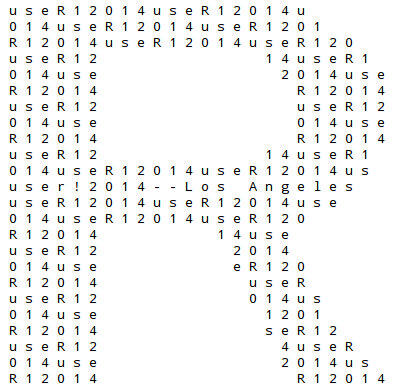
R[265:286]<-strsplit('user!2014--Los Angeles', '')[[1]]

R<-data.frame(matrix(R,ncol=24, byrow=T))
names(R) = rep(' ', ncol(R))
print(R, row.names=F)
# write.table(R, file="tshirtImage.txt", quote=FALSE)

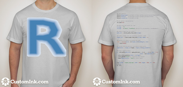
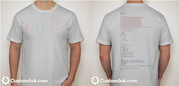
Generated image

T-shirt with highlighted code

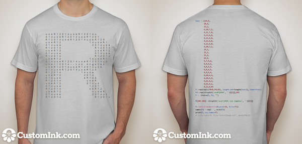
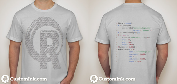
#2 by @daroczig: using pixmap to create ASCII art

As the code will be printed on the t-shirt, maybe it would look cooler with some shorter codebase by using an R package instead of a long, manually defined numeric vector. This also results in a higher resolution ASCII art, although the matrix of course can be reduced.

This pull request has several alternate solutions, here goes a quick list of those and a quick demo of the last one:

Code

library(pixmap)

## get R logo into a matrix
R <- read.pnm(
    system.file('pictures/logo.ppm',
                package = 'pixmap')[1])

## drop colors
R <- addChannels(R)@grey

## create a matrix full of "useR! 2014"
T <- matrix(
    strsplit('useR!2014', '')[[1]],
    nrow = nrow(R),
    ncol = ncol(R),
    byrow = TRUE)

## remove cells not in the R logo
T[which(R > 0.85)] <- ' '

## save to disk
write.table(x = T, # never abbreviate TRUE to T :)
            file = 'tshirtImage.txt',
            row.names = FALSE,
            sep = '',
            col.names = FALSE,
            quote = FALSE)

Generated image

T-shirt with highlighted code

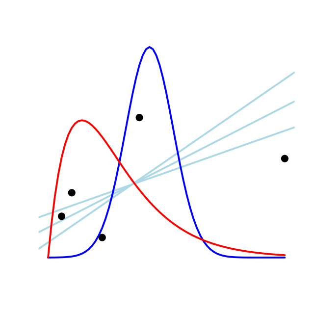
#3 by @bryanhanson: Bayes Icon

Code

# Bayes Icon Idea
# Inspired by
# http://doingbayesiandataanalysis.blogspot.com/2013/12/icons-for-essence-of-bayesian-and.html
# Bryan Hanson, DePauw University, Greencastle Indiana USA
# May 16, 2014

# This is all fake data designed as a talking point, 
# and suited to be a logo that prints
# well in a limited range of colors, like on a t-shirt!

x1 <- seq(0, 7, by = 0.1) # faux priors/distributions
y1 <- exp(-(x1-3)**2)/sqrt(pi)
y2 <- x1*exp(-x1)

set.seed(7) # faux data points
ns <- 5
x3 <- sample(x1, ns)
y3 <- rnorm(ns, mean = 0.5*diff(range(y2)), sd = 0.1)

mod <- lm(y3~x3) # fit a line

nl <- 3 # faux set of slopes
noise <- rnorm(nl, sd = 0.04)
i <- mod$coef[1] + noise
df <- data.frame(x = 0, y = i)

# empty plot region
plot(x1, y1, type = "n", axes = FALSE, ylab = "", xlab = "")

mods <- list() # add the slopes
for (n in 1:nl) {
    x = c(mean(x3), 0)
    y = c(mean(y3), i[n])
    mods[[n]] <- lm(y~x)
    abline(mods[[n]], lwd = 5, col = "lightblue")
    }

# add the points and distributions
lines(x1, y1, type = "l", col = "blue", lwd = 5)
lines(x1, y2, col = "red", lwd = 5)
points(x3, y3, pch = 20, cex = 3)

Generated image

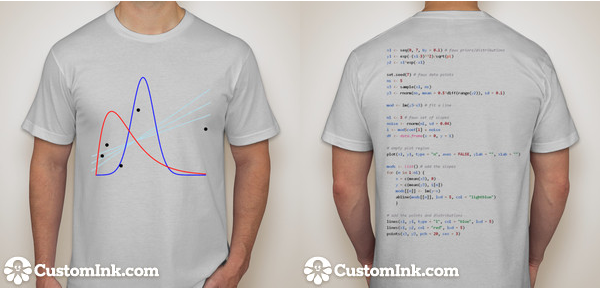
T-shirt with highlighted code

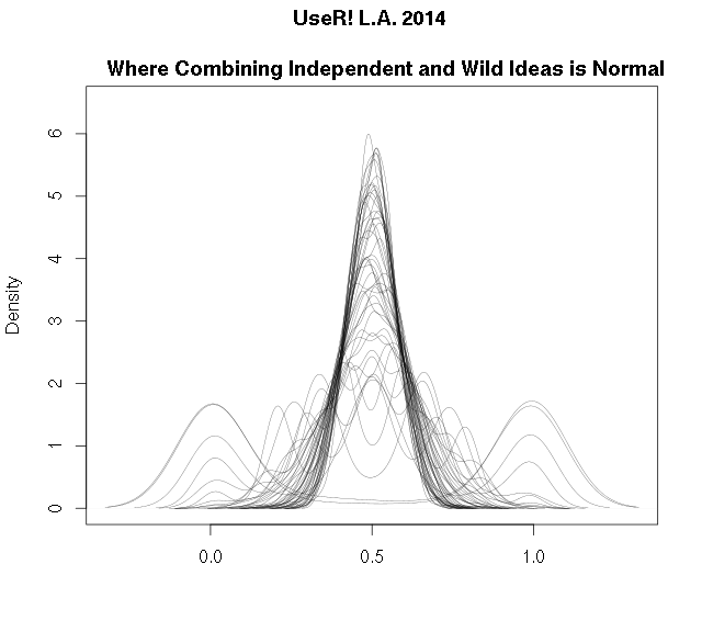
#4 by @fhoces: CLT with R

Very simple demonstration of the CLT using k betas(0.05,0.05). I'm pretty basic about the graphics so any suggestions are welcome.

Code

dev.off()
set.seed(20140630)

clt = function(n,k) apply(matrix(rbeta(n*k,.05,.05),n, k), 1, sum)/k
plot(density(clt(1000,1)), lwd=.3, ylim=c(0,6.5), main="UseR! L.A. 2014 \n 
Where Combining Independent and Wild Ideas is Normal", xlab="") 
sapply(1:50, function(x) lines(density(clt(1000,x)), lwd=.3, xlab=""))

Generated image

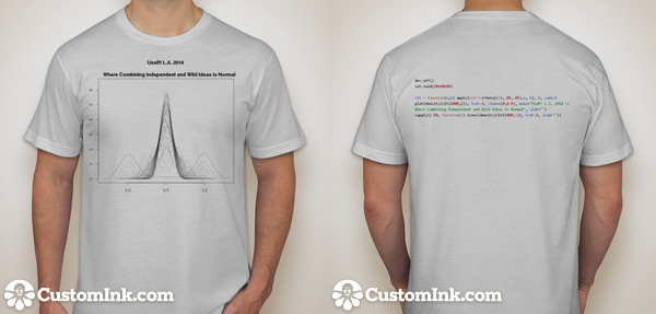
T-shirt with highlighted code

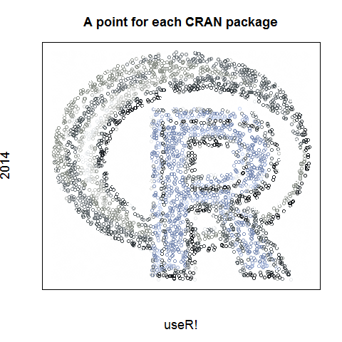
#5 by @MarkTPatterson: EBImage package

Code

# Script by Mark T Patterson
# May 17, 2014
# twitter: @M_T_Patterson

# General Notes:

# This script creates an image of the R logo 
# represented by n points, 
# where n is the current number of packages on CRAN


# note: this script requries the EBImage package
# available from bioconductor:
# http://bioconductor.wustl.edu/bioc/html/EBImage.html

# approximate run time: 2 mins

#### initialize ####

# clear workspace
rm(list = ls())


# load libraries
library(EBImage) 

# coordinate the version of the program:
set.seed(2014)

#### gather web data: reference image and CRAN package count ####

# load the R logo, save the rgb values:
img = readImage("http://www.thinkr.spatialfiltering.com/images/Rlogo.png")
img.2 = img[,,1:3]

cran.site = "http://cran.r-project.org/web/packages/"
lns = readLines(cran.site)
ref.line = grep(lns, pattern = "CRAN package repository features")
package.count = as.numeric(strsplit(lns[ref.line],split = "\\s")[[1]][7])


#### helper functions ####

# functions for color simplification:
num.to.let = function(x1){
  ref.dat = data.frame(num = 10:15, let = LETTERS[1:6])
  out = as.character(x1)
  if(x1 %in% 10:15){out = as.character(ref.dat$let[which(ref.dat$num == x1)])}
  return(out)
}

rgb.func = function(vec){
  #note: vec is a triple of color intensities
  r1 = floor(255*vec[1])
  g1 = floor(255*vec[2])
  b1 = floor(255*vec[3])
  
  x1 = r1 %/% 16
  x2 = r1 %% 16
  x3 = g1 %/% 16
  x4 = g1 %% 16
  x5 = b1 %/% 16
  x6 = b1 %% 16
  
  x1 = num.to.let(x1)
  x2 = num.to.let(x2)
  x3 = num.to.let(x3)
  x4 = num.to.let(x4)
  x5 = num.to.let(x5)
  x6 = num.to.let(x6)
  
  out = paste("#",x1,x2,x3,x4,x5,x6, sep = "")
  return(out)
  
}


im.func.1 = function(image, k.cols = 5, samp.val = 3000){
  # creating a dataframe:
  test.mat = matrix(image,ncol = 3)
  df = data.frame(test.mat)
  colnames(df) = c("r","g","b")
  df$y = rep(1:dim(image)[1],dim(image)[2])
  df$x = rep(1:dim(image)[2], each = dim(image)[1])
  
  samp.indx = sample(1:nrow(df),samp.val)
  work.sub = df[samp.indx,]
  
  # extracting colors:
  k2 = kmeans(work.sub[,1:3],k.cols)
  
  # adding centers back:
  fit.test = fitted(k2)
  
  work.sub$r.pred = fit.test[,1]
  work.sub$g.pred = fit.test[,2]
  work.sub$b.pred = fit.test[,3]
  
  return(work.sub)
  
}

add.cols = function(dat){
  apply(dat,1,rgb.func)
}

# general plotting function
plot.func = function(dat){
  # assumes dat has colums x, ym cols
  plot(dat$y,max(dat$x) - dat$x, col = dat$cols, 
       main = "A point for each CRAN package",
       xaxt='n',
       yaxt="n",
       xlab = "useR!",
       ylab = "2014",
       cex.lab=1.5, 
       cex.axis=1.5, 
       cex.main=1.5, 
       cex.sub=1.5)
}

#### simplify colors; sample n points ###

temp = im.func.1(img.2, samp.val = 25000, k = 12)
temp$cols = add.cols(temp[,6:8])

final = temp[sample(1:nrow(temp), package.count),]


#### generate plot ####

plot.func(final)

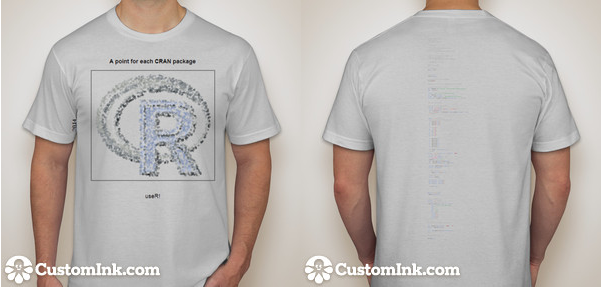
Generated image

T-shirt with highlighted code

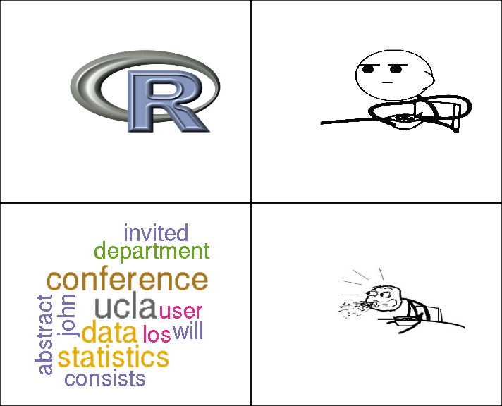
#6 by @calycolor: wordcloud

Sometimes I am so amazed by the visuals created in R that I feel like I am blowing my cereal :)

Code

# jo f. with thanks to:
# http://is-r.tumblr.com/post/46821313005/to-plot-them-is-my-real-test
# http://stackoverflow.com/questions/12918367/in-r-how-to-plot-with-a-png-as-background
# http://students.washington.edu/mclarkso/documents/figure%20layout%20Ver1.R
# http://georeferenced.wordpress.com/2013/01/15/rwordcloud/

rm(list=ls())
sapply(c("stringr", "jpeg", "RCurl", "EBImage", "wordcloud", "tm"),library, character.only=TRUE)
allImageURLs <- c("http://upload.wikimedia.org/wikipedia/commons/c/c1/Rlogo.png",
                  "http://www.memes.at/faces/cereal_guy_squint.jpg",
                  "http://img2.wikia.nocookie.net/__cb20120912234733/ragecomic/images/9/91/Cereal_Guy_Spitting.jpeg")
imageList <- list()
for(imageURL in allImageURLs) {
    print(imageURL)
   tempName <- str_extract(imageURL,"([[:alnum:]_-]+)([[:punct:]])([[:alnum:]]+)$")
   print(tempName)
   tempImage <- readImage(imageURL) 
   imageList[[tempName]] <- tempImage 
}
par(mfrow=c(2,2))  
plot(0:10, 0:10, type="n", axes=F, ann=FALSE)
rasterImage(imageList[[1]],1,1,10,10)
box("figure", col="black", lwd=2)
plot(0:10, 0:10, type="n", axes=F, ann=FALSE)
rasterImage(imageList[[2]],1,1,10,10)
box("figure", col="black", lwd=2)
useR <- Corpus (DirSource("./useRdir"))
useR <- tm_map(useR, stripWhitespace)
useR <- tm_map(useR, tolower)
useR <- tm_map(useR, removeWords, stopwords('english'))
wordcloud(useR, scale=c(4,1.25), max.words=100, random.order=FALSE, rot.per=0.35, use.r.layout=FALSE, colors=brewer.pal(8,'Dark2'))
box("figure", col="black", lwd=2)
plot(0:10, 0:10, type="n", axes=F, ann=FALSE)
rasterImage(imageList[[3]],1,1,10,10)
box("figure", col="black", lwd=2)

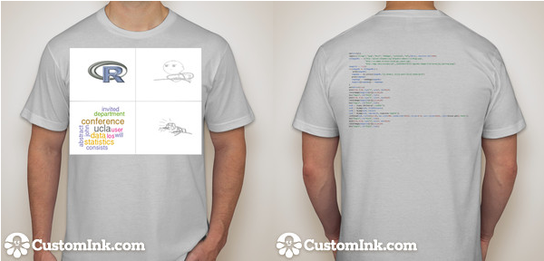
Generated image

T-shirt with highlighted code

#8 by @woobe: RShapeTarget package

My first attempt based on Pierre's examples in his package "RShapeTarget". Two designs. Note: this is also my first ever pull request :) See you in LA!

Code

## Load libraries
library(RShapeTarget) # available on https://github.com/pierrejacob/RShapeTarget/
library(rPlotter)     # availalbe on https://github.com/woobe/rPlotter
library(wesanderson)  # available on CRAN

## Set seed for reproducibility
set.seed(1234)

## Define word and colours for logo
txt_logo <- "R"
col_logo <- c("white", "steelblue")  ## Also try wes.palette(4, "GrandBudapest")

## Create a shape from the letter R
path_word <- extract_paths_from_word(txt_logo)

## Create a target with some smoothness parameter lambda
target_word <- create_target_from_word(txt_logo, lambda = 1)

## Generate in a square surrounding the shape
rinit <- function(size)  csr(target_word$bounding_box, size)
x <- rinit(200000)

## Evaluate the log densities associated to these points
logdensities <- target_word$logd(x, target_word$algo_parameters)

## Create a ggplot2 object
g <- plot_paths(path_word) + geom_point(aes(x = x[,1], y = x[,2], alpha = 0.01,
                                            colour = exp(logdensities))) +
  scale_colour_gradientn(colours = col_logo) +
  create_ggtheme("blank") +  # function from rPlotter
  theme(legend.position = "none") # remove legend

## Save as PNG
png(filename = "output_logo.png", width = 2000, height = 2000, res = 300)
print(g)
dev.off()

Generated image

T-shirt with highlighted code

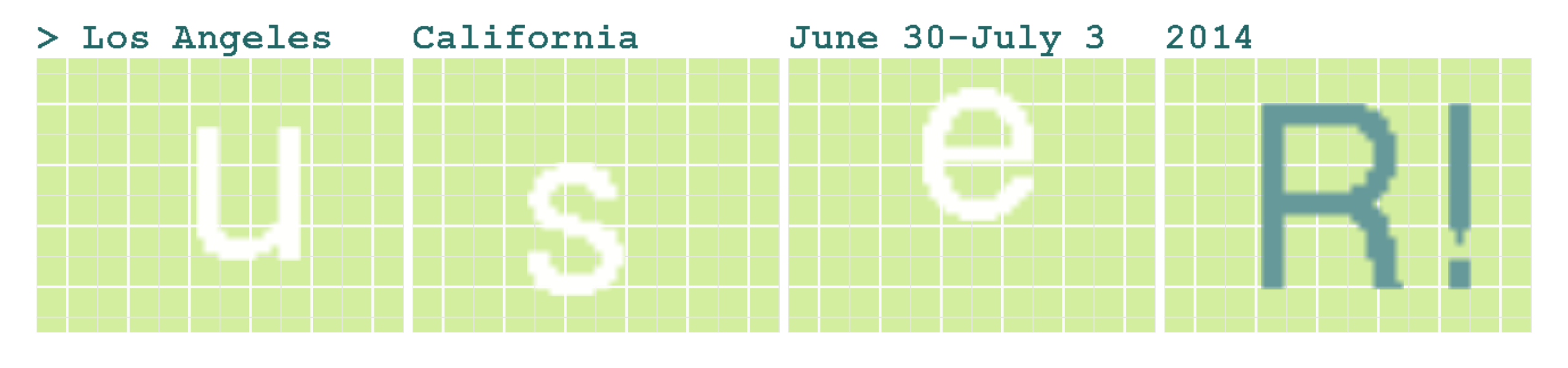
#9 by @hanel: ggplot2

I added a simple ggplot2 t-shirt image.

Code

library(ggplot2)
library(grid)

event = data.frame(
  
  DETAILS = c('> Los Angeles', 'California', 'June 30-July 3','2014'),
  NAME = c('u','s','e','R!'), 
  COLOR = factor(c(1, 1, 1, 2), levels = c(1, 2))
  
)

event$DETAILS = factor(event$DETAILS, levels = event$DETAILS)

set.seed(2014)

ggplot(event) + 
  geom_text(aes(x = 0, y=0, label=NAME, color = COLOR,hjust = rnorm(4, 0.5, .2), vjust = rnorm(4, 0.5, .2)), size = rel(35), face = 'bold') + 
  facet_grid(~DETAILS) +
  theme_bw() +
  theme(axis.title = element_blank(), 
        axis.text = element_blank(), 
        axis.ticks = element_blank(), 
        strip.text = element_text(hjust = 0, size = rel(1.25), face = 'bold', color = '#226666', family='mono'),
        strip.background = element_rect(fill = 'white', colour = 'white'),
        panel.background = element_rect(fill = ('#D3EE9E')), 
        panel.border = element_blank(), 
        plot.margin = unit(c(-0.5,1,-1,0), 'lines')) +
  coord_fixed(xlim = c(-3, 3), ylim = c(-2.25, 2.25)) +
  scale_color_manual(guide='none', values = c('#FFFFFE', '#669999'))

ggsave('tshirtImage.png', width = 8.5, height = 2)

Generated image

T-shirt with highlighted code

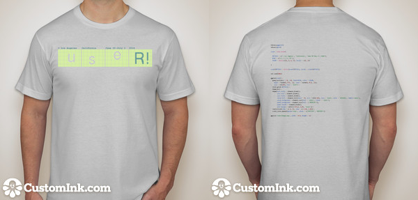
#10 by @royfrancis: RShapeTarget package

Code

#useR! Design R Script

#load libraries
require(ggplot2)
require(RColorBrewer)
require(Cairo)

#create number of repeats
pos <- c(60,13,14,5,60,17,10,5,63,5,5,5,9,5,63,4,7,5,8,5,63,4,8,4,8,4,64,4,8,5,7,4,64,3,10,4,7,4,64,3,10,4,6,4,64,4,10,4,6,4,64,4,10,4,6,4,7,3,11,2,9,5,12,5,10,4,9,4,7,4,6,4,9,3,9,7,9,8,9,3,10,4,7,3,5,6,9,3,7,2,3,4,7,3,4,4,8,3,9,4,8,3,4,2,1,4,9,3,6,2,6,2,6,3,5,4,7,4,9,4,8,3,3,2,2,3,9,4,6,2,13,3,6,4,7,4,8,4,9,2,8,3,9,4,5,3,12,3,7,4,7,4,6,4,11,2,8,3,9,3,6,3,12,3,7,3,8,12,12,3,7,4,9,3,6,4,10,3,7,3,9,12,12,3,7,3,10,3,6,5,9,3,5,4,9,4,5,4,12,2,8,3,9,4,7,6,6,4,3,4,11,4,5,5,11,2,8,3,8,4,9,6,5,9,13,4,6,4,11,2,7,4,8,4,10,6,4,6,16,4,6,4,11,2,7,4,7,5,11,5,4,3,19,3,8,4,19,3,7,6,12,5,3,3,18,4,8,4,19,3,6,2,1,4,13,4,2,4,18,4,8,5,18,3,5,2,2,3,15,3,2,4,18,4,9,5,16,4,4,2,3,3,3,1,11,3,3,4,9,2,6,4,9,5,6,3,7,4,3,2,4,3,2,2,1,3,7,2,4,4,8,2,7,4,10,5,4,5,6,4,2,2,4,7,2,4,5,3,4,5,5,3,7,5,11,4,4,5,6,7,5,6,3,6,2,3,5,11,8,6,11,5,3,5,6,6,6,5,5,8,8,9,6,12,10,5,1,5,7,3,9,2,8,5,12,4,9,12,13,2,1,4,6)
#create 1s and 0s using repeats
d1 <- rep(rep(c(1,0), length.out=length(pos)), times=pos)
#convert to matrix
d2 <- data.frame(matrix(d1,ncol=92, byrow=T))
#get x coord, y coord and z values
yvec<-vector()
xvec<-vector()
zvec<-vector()
for(i in 1:nrow(d2))
{
  for(j in 1:ncol(d2))
  {
    yvec<-c(yvec,i)
    xvec<-c(xvec,j)
    zvec<-c(zvec,d2[i,j])
  }
}

#create dataframe
d3 <- data.frame(x=xvec,y=yvec,z=zvec)
#remove value 1
d4<-subset(d3,d3$z==0)
#jitter coordinates
d4$x <- jitter(d4$x,4,0.5)
d4$y <- jitter(d4$y,4,0.5)
d4$x1 <- jitter(d4$x,4,0.5)
d4$y1 <- jitter(d4$y,4,0.5)
#random size in 2 layers to increase density
d4$size<-sample(1:9,nrow(d4),replace=T)
d4$size1<-sample(9:16,nrow(d4),replace=T)
#random alpha variation
d4$alpha<-sample(2:4,nrow(d4),replace=T)/10
d4$alpha1<-sample(4:9,nrow(d4),replace=T)/10

#plotting
p<-ggplot()+
  geom_point(data=d4,aes(x=x,y=y,col=x,size=size,alpha=alpha),shape="+")+
  geom_point(data=d4,aes(x=x1,y=y1,col=x,size=size1,alpha=alpha1),shape="+")+
  scale_colour_gradientn(colours= brewer.pal(5,"Set1"),space ="rgb",guide=FALSE)+
  scale_y_reverse()+
  theme_minimal()+
  labs(x="",y="")+
  theme(legend.position="none",axis.text=element_blank(),axis.ticks=element_blank(),panel.grid=element_blank())

#export image #maintain aspect ratio around 1:3
png("useR.png",height=10,width=30,res=200,units="cm",type="cairo")
print(p)
dev.off()

Generated image

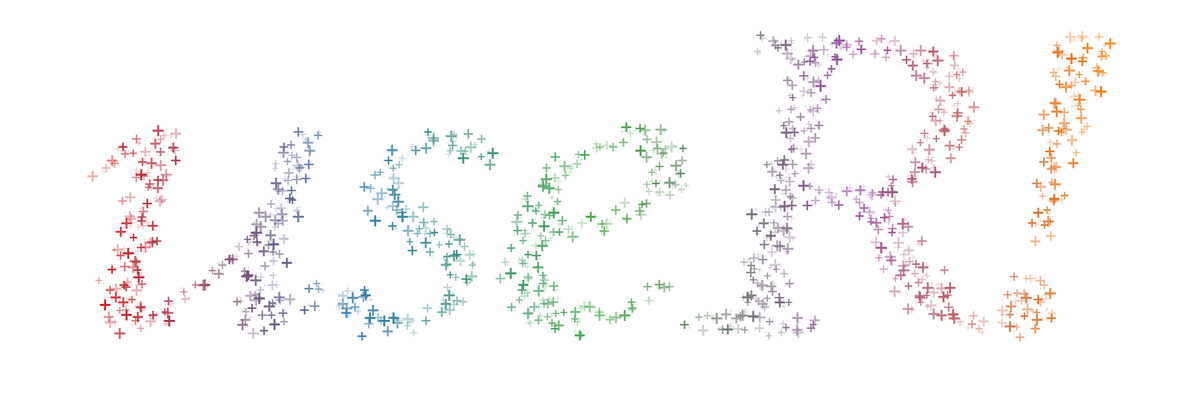
T-shirt with highlighted code

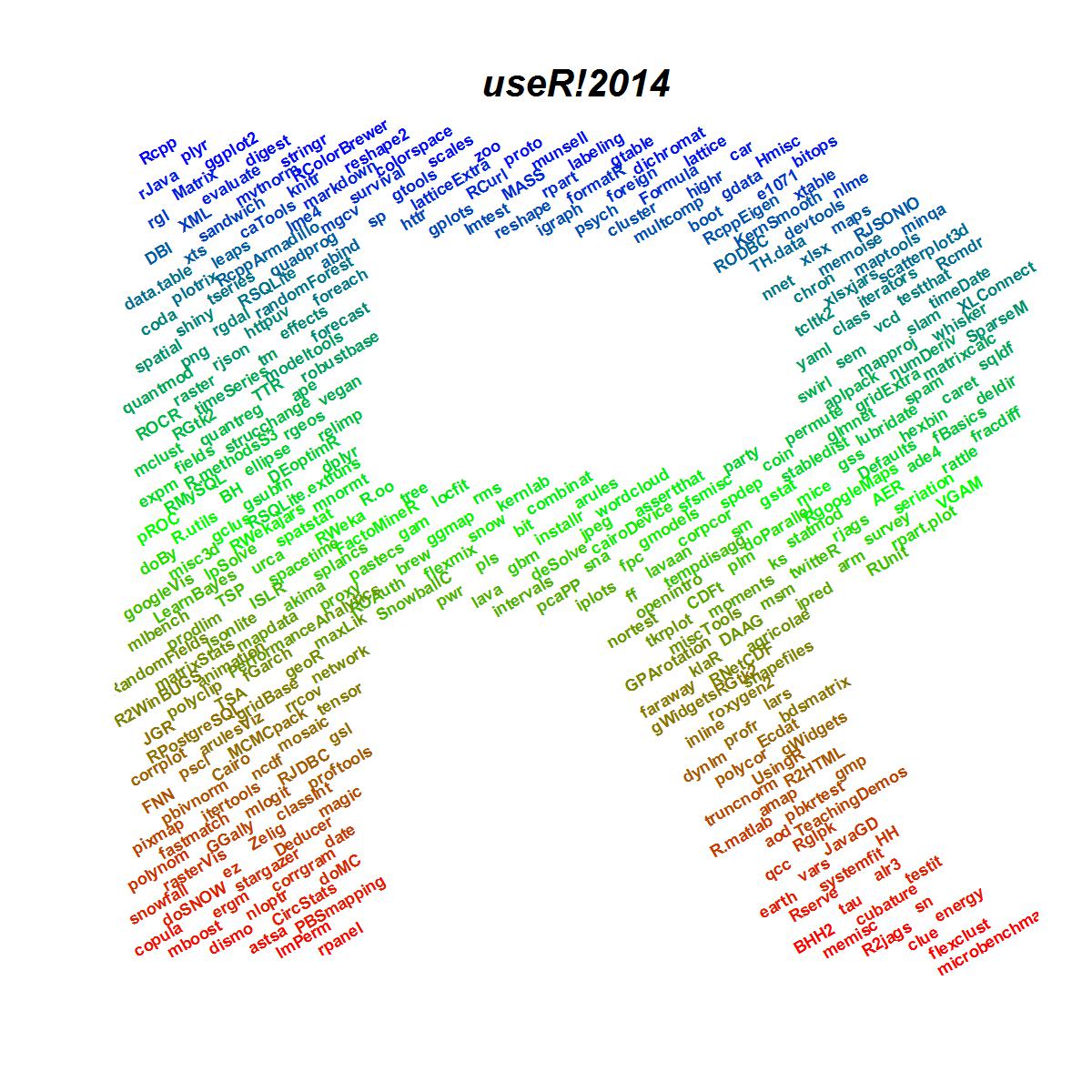
#11 by @notesofdabbler

I wanted to make an attempt building on some of the entries already made. Specifically, I used the first version that had R with letters user2014 and created a version where the letter R is made up of top downloaded R packages (that form the backbone of R). The figure is rough on the edges and the code is a bit too long. Nevertheless, I am putting it here if some aspect of this is found useful by others coming up with more entries.

Code

# load libraries
library(ggplot2)
library(scales)


# set working directory
setwd("~/notesofdabbler/t-shirt/")


# code taken from github initial commit 
R<-c(rep(1,19),rep(0,5),rep(1,20),rep(0,4),rep(1,22),rep(0,2),rep(1,6),rep(0,10),rep(1,7),0,
     rep(1,6),rep(0,11),rep(1,7),rep(1,6),rep(0,12),rep(1,6),rep(1,6),rep(0,12),rep(1,6), 
     rep(1,6),rep(0,12),rep(1,6),rep(1,6),rep(0,12),rep(1,6),rep(1,6),rep(0,10),rep(1,7),0,
     rep(1,23),0,rep(1,22),rep(0,2),rep(1,21),rep(0,3),rep(1,19),rep(0,5),
     rep(1,6),rep(0,7),rep(1,5),rep(0,6),rep(1,6),rep(0,8),rep(1,4),rep(0,6),
     rep(1,6),rep(0,8),rep(1,5),rep(0,5),rep(1,6),rep(0,9),rep(1,4),rep(0,5),
     rep(1,6),rep(0,9),rep(1,5),rep(0,4),rep(1,6),rep(0,10),rep(1,4),rep(0,4),
     rep(1,6),rep(0,10),rep(1,5),rep(0,3),rep(1,6),rep(0,11),rep(1,5),rep(0,2),
     rep(1,6),rep(0,11),rep(1,6),rep(0,1),rep(1,6),rep(0,12),rep(1,6))

# Create x and y coordinates for plotting letter R
Rx=rep(seq(1,24),24)
Ry=rep(seq(24,1),each=24)
# data for plotting letter R is gathered into a data frame
df=data.frame(R=R,Rx=Rx,Ry=Ry)
# rows with R=0 are not part of the plot
df=subset(df,R==1)
# test of graph with just points
#ggplot(data=df,aes(x=Rx,y=Ry))+geom_point(size=4)

#---------------Finding top downloaded CRAN packages during 3 months (Feb-Apr 2014)-----------------------
# This piece of code is from http://www.nicebread.de/finally-tracking-cran-packages-downloads/  

## ======================================================================
## Step 1: Download all log files
## ======================================================================

# Here's an easy way to get all the URLs in R
start <- as.Date('2014-02-01')
today <- as.Date('2014-04-30')

all_days <- seq(start, today, by = 'day')

year <- as.POSIXlt(all_days)$year + 1900
urls <- paste0('http://cran-logs.rstudio.com/', year, '/', all_days, '.csv.gz')

# only download the files you don't have:
missing_days <- setdiff(as.character(all_days), tools::file_path_sans_ext(dir("CRANlogs"), TRUE))

dir.create("CRANlogs")
for (i in 1:length(missing_days)) {
  print(paste0(i, "/", length(missing_days)))
  download.file(urls[i], paste0('CRANlogs/', missing_days[i], '.csv.gz'))
}

## ======================================================================
## Step 2: Load single data files into one big data.table
## ======================================================================

file_list <- list.files("CRANlogs", full.names=TRUE)

logs <- list()
for (file in file_list) {
  print(paste("Reading", file, "..."))
  logs[[file]] <- read.table(file, header = TRUE, sep = ",", quote = "\"",
                             dec = ".", fill = TRUE, comment.char = "", as.is=TRUE)
}

# rbind together all files
library(data.table)
dat <- rbindlist(logs)

# delete the CRANlogs directory
unlink("CRANlogs",recursive=TRUE)

# find number of downloads of packages
library(dplyr)
pkgcount=dat%>%group_by(package)%>%summarize(downloads=n())%>%arrange(desc(downloads))
# check top 25
#head(pkgcount,25)

#---------------plot letter R with top downloaded package names instead of points-----------------

# number of points in R letter
numptsR=nrow(df)

# The current R letter plot has 342 points
# Extract top 342 downloaded packages
pkgcountTop=pkgcount[1:numptsR,]

# Add info on top packages to dataframe with R letter coordindates
df$package=pkgcountTop$package
df$pkgcount=pkgcountTop$count
df$colornum=seq(1,numptsR) # here just a rank ordering is used for coloring

ggplot(data=df,aes(x=Rx,y=Ry))+
  geom_text(aes(label=package,angle=30,color=as.numeric(colornum)),size=1.5,fontface="bold")+
  theme_bw()+
  theme(axis.ticks=element_blank(),axis.text=element_blank(),legend.position="none",
        plot.background = element_blank(),panel.grid.major = element_blank(),
        panel.grid.minor = element_blank(),panel.border = element_blank())+
  xlab("")+ylab("")+scale_color_gradient2(low="blue",mid="green",high="red",midpoint=floor(numptsR/2))+
  ggtitle("useR!2014")+theme(plot.title=element_text(face="bold.italic",size=10))

ggsave("user2014_tShirt_entry.jpg",width=4,height=4)